How to Use Benchmarks

OptunaHub provides various benchmarks, and you can utilize them through a unified interface. In this tutorial, we will explain how to use benchmarks in OptunaHub. If you are interested in registering your own benchmark problems, please check Basic and Advanced tutorials.

The following blog post also provides an overview of this feature:

OptunaHub Benchmarks: A New Feature to Use/Register Various Benchmark Problems

Preparation

First, ensure the necessary packages are installed by executing the following command:

$ pip install optuna optunahub

Examples

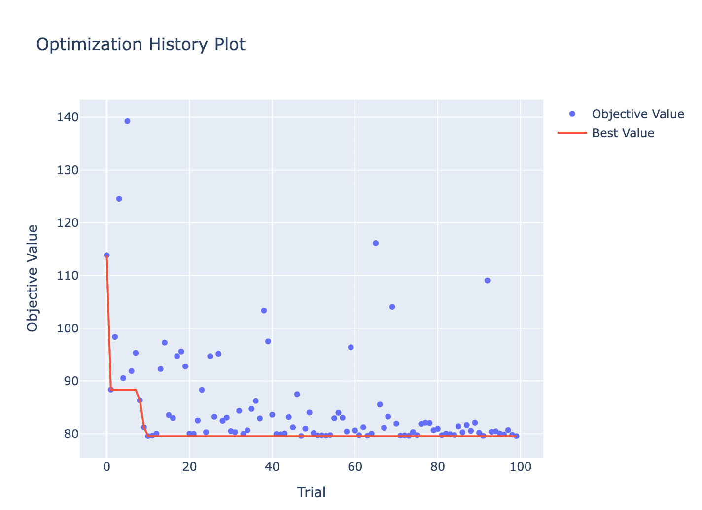
We will use the black-box optimization benchmarking (bbob) test suite in this tutorial. This is a wrapper of COCO (COmparing Continuous Optimizers) experiment library. So you need to install COCO first.

$ pip install coco-experiment

Test code is as follows:

import optuna
import optunahub


bbob = optunahub.load_module("benchmarks/bbob")
sphere2d = bbob.Problem(function_id=1, dimension=2, instance_id=1)

study = optuna.create_study(directions=sphere2d.directions, sampler=optuna.samplers.TPESampler(seed=42))
study.optimize(sphere2d, n_trials=100)

optuna.visualization.plot_optimization_history(study).show()

You can also use other optimizing frameworks to optimize the problem. BaseProblem provides __call__() and evaluate() methods, which is used to evaluate the objective function. __call__() takes an optuna.Trial object, while evaluate() takes a dictionary of input parameters. Therefore, you can use evaluate() to optimize the problem with other optimizing frameworks. Here, we use scipy.optimize.minimize as an example. The properties initial_solution, lower_bounds, and upper_bounds are provided by the bbob package.

import optunahub
import scipy


bbob = optunahub.load_module("benchmarks/bbob")
sphere2d = bbob.Problem(function_id=1, dimension=2, instance_id=1)
result = scipy.optimize.minimize(
    fun=lambda x: sphere2d.evaluate({f"x{d}": x[d] for d in range(sphere2d.dimension)}),
    x0=sphere2d.initial_solution,
    bounds=scipy.optimize.Bounds(
        lb=sphere2d.lower_bounds, ub=sphere2d.upper_bounds
    )
)

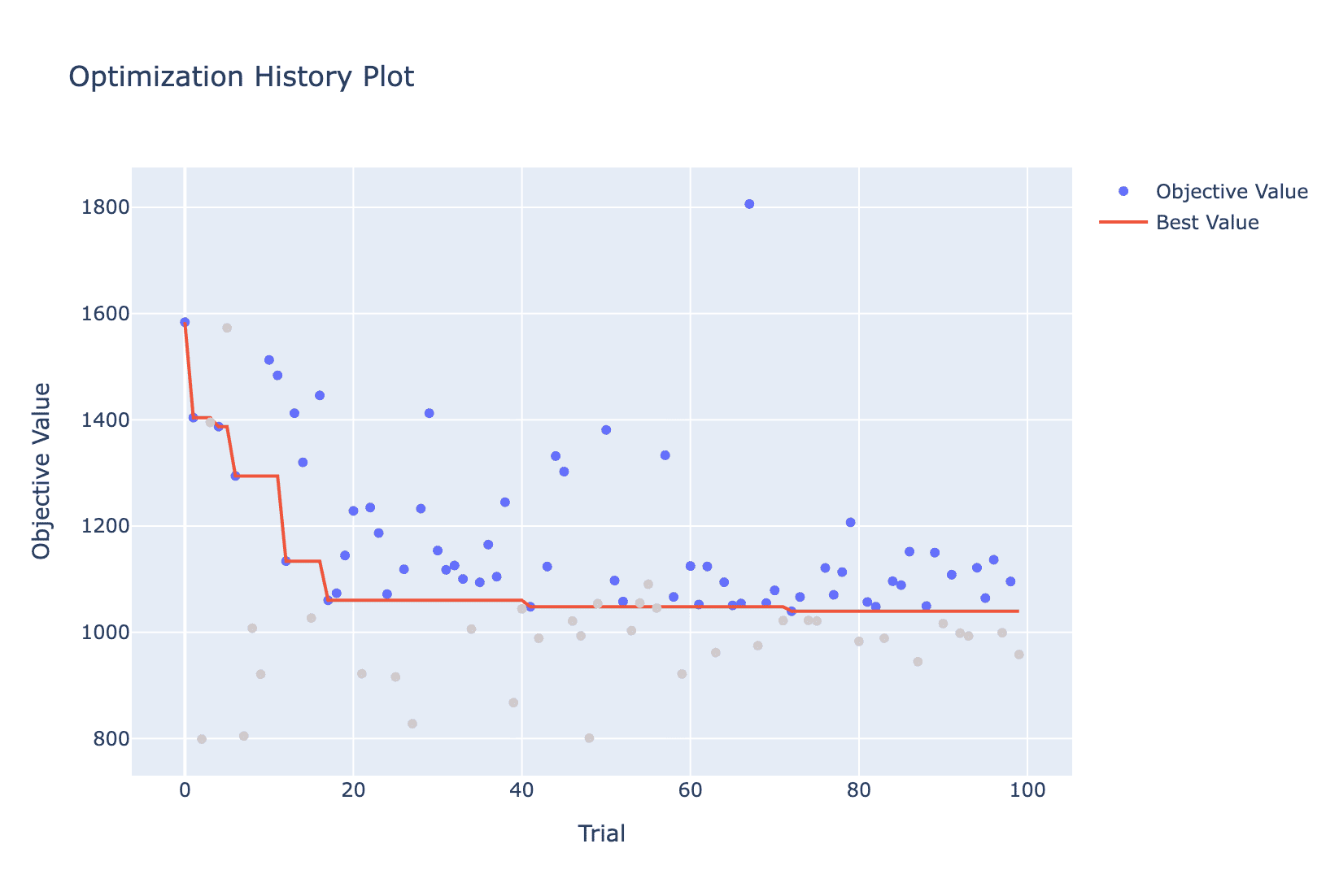
Constrained Problem

Some benchmarks also include constraints. These problems are implemented by inheriting ConstrainedMixin class. ConstrainedMixin provides evaluate_constraints() and constraints_func() methods. As same as objective functions, constraints_func() takes an optuna.Trial object, while evaluate_constraints() takes a dictionary of input parameters. Those methods are used to evaluate the constraint functions. You can optimize these problems in the same way as usual, but you need to set the constraints_func argument in the sampler.

import optuna
import optunahub
import matplotlib.pyplot as plt

bbob_constrained = optunahub.load_module("benchmarks/bbob_constrained")
constrained_sphere2d = bbob_constrained.Problem(function_id=1, dimension=2, instance_id=1)

study = optuna.create_study(
    sampler=optuna.samplers.TPESampler(
        constraints_func=constrained_sphere2d.constraints_func,
        seed=42
    ),
    directions=constrained_sphere2d.directions
)
study.optimize(constrained_sphere2d, n_trials=100)
optuna.visualization.plot_optimization_history(study).show()
plt.show()

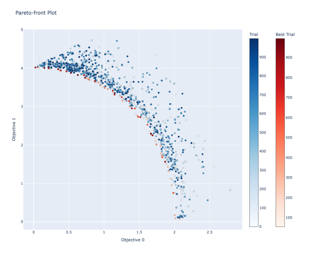
Multi-Objective Problem

You can also try multi-objective optimization. Here, we use the the WFG Problem Collection as an example. In order to use this module, you need to install optproblems and diversipy packages.

$ pip install -U optproblems diversipy

Example is as follows:

import optuna
import optunahub


wfg = optunahub.load_module("benchmarks/wfg")
wfg4 = wfg.Problem(function_id=4, n_objectives=2, dimension=3, k=1)

study = optuna.create_study(
    study_name="TPESampler",
    sampler=optuna.samplers.TPESampler(seed=42), directions=wfg4.directions
)
study.optimize(wfg4, n_trials=1000)

optuna.visualization.plot_pareto_front(study).show()

Keep Exploring!

There are many kinds of benchmarks in OptunaHub. You can find them in the OptunaHub Benchmarks page.